The problem with perfect phylogenies

9 minute read

Previously, I wrote a blog post, exploring the Gusfield algorithm for building phylogenetic trees from binary traits. While the algorithm works well if you have a clean matrix that just-so happens to form a perfect phylogeny, if you experiment with different matrix permutations of 1s and 0s, you’ll quickly find that matrices which create perfect phylogenies are scarce. Indeed, if there are any pairs of columns [C1,C2] that have the values [0,1], [1,0] and [1,1], then a perfect phylogeny cannot be built. Imperfect data sources and noisy data can contribute to the difficulties of building a valid phylogeny. To allow for some slack for running the phylogeny-finding algorithm, one option is to use the imperfect phylogeny algorithm, which is described (and implemented in near-linear time) in a paper by Pe’er et al. (pay-walled, unfortunately). I will explain and implement this algorithm in code in this post. If you’re after the mathematical proofs or description, refer to the original paper.

A motivation for using the imperfect phylogeny algorithm

In modelling phylogenetic trees from binary data, it is unlikely that you’ll have absolute certainty in observing data values. In my early experiments of my PhD project, I was utilising the Gusfield algorithm for structural variation (SV) data in multiple tumour biopsies from the same patient. In my case, observing the same structural variation across several tumour samples of the same patient gave me high confidence that the variation existed. However, I was much less confident when I did not see variant in one patient sample, when it was clearly present in others. Thus, my ‘1’s were certain, but my ‘0’s were uncertain. In the case of structural variants, there are several reasons why we might not detect a variant in a particular sample (the depth of coverage may be too low, or the sample may have a low amount of tumour content). In this case, when I constructed my matrix of shared SV events, I would mark the rows of my low-quality samples with ‘incomplete/unknown’ values to represent this uncertainty. This strategy allowed me to find valid phylogenies where previously they could not be found.

The incomplete phylogeny problem

In our feature matrix, we now allow a third feature type - unknown or incomplete, denoted by ‘?’. Hence our values can be 0, 1 or ? for any cell. The incomplete phylogeny algorithm will then infer the unknown values by determining whether the sample belongs to the ‘clade’ associated with the feature - the clade being the evolutionary group with a common ancestor, that the sample/species evolved from.

The algorithm will output a perfect phylogeny tree T (if present), as well as the corresponding completed matrix M. The algorithm is composed of the following steps:

Remove any columns in our matrix M with no 0s or all 0s.
Construct a graph where 1s represent edges between features (columns) and samples (rows).
Get each set of connections where there are >1 connections (call these K) in the graph G, for each K (while G \neq \emptyset):

i. get all the samples (S or rows) in K, call this S’.

ii. for this set of S’, get all the features (C or columns) where there are no 0 entries, call this U.

iii. if there are no elements in U, stop.

iv. otherwise remove U from the graph G (also removing any connections), and add S’ to our tree T.
For any Cs that are associated with the clade S, set these to 1, otherwise 0.
Return T and M’.

The vector T now represents our phylogenetic tree. This represents the clades that are present in our tree. For instance, if T = {{s1,s2,s3,s4},{s1,s2},{s3,s4}}, this means that our ‘super-clade’ has 4 elements, {s1,s2,s3,s4}, and two clades consisting of {s1,s2} and {s3,s4}, which are more closely related than the other pairs. The tree could be drawn as:

                                    /\
                                   /  \
                                  /    \
                                 /\    /\
                                /  \  /  \
                               s2 s2  s3 s4

To implement the algorithm, Let’s work from the following matrix (already sorted by its binary values, see previous post for more info):

	C1	C2	C3	C4	C5
S1	1	1	0	0	?
S2	0	?	1	0	?
S3	1	?	0	0	1
S4	0	0	1	1	?
S5	0	1	0	0	?

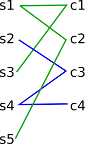
We will now transform this matrix into a graph, creating connections between the nodes, Cs and Ss. Edges are defined where C and S share a value of ‘1’. To do this, we first code up an graph implementation, with nodes and edges. The base graph code, as well as the M Graph implementation are in the mgraph.py file.

We now build our arrays for our Ss and Cs, as well as or M matrix. Let’s use -1 to represent the ‘incomplete’ state of our matrix.

from mgraph import MGraph
import numpy as np

s = np.array(['s1','s2','s3','s4','s5'])
c = np.array(['c1','c2','c3','c4','c5'])
m = np.array([[ 1,  1,  0,  0, -1],
              [ 0, -1,  1,  0, -1],
              [ 1, -1,  0,  0,  1],
              [ 0,  0,  1,  1, -1],
              [ 0,  1,  0,  0, -1]])

# create working matrix M and column C vector copies
m3 = m.copy()
c3 = c.copy()

# remove any columns where there are no 0 entries
mi = np.empty(0,dtype='int')
ncol = len(m3[0])
idxs_to_delete = [i for i in range(ncol) if not np.any(m3[:,i:i+1]==0)]
m3 = np.delete(m3,idxs_to_delete,axis=1)
c3 = np.delete(c3,idxs_to_delete)

m_graph = MGraph()
m_graph.build_graph(m3,s,c3)
m_pairs = m_graph.get_edge_pairs()

print('Nodes in our graph')
print(m_graph.getNodes())

print('\nPairwise connections between out nodes')
print(m_graph.get_edge_pairs())

Which returns the output:

Nodes in our graph
['s3', 's2', 's1', 's5', 's4', 'c3', 'c2', 'c1', 'c4']

Pairwise connections between out nodes
[['s3', 'c1'], ['s2', 'c3'], ['s1', 'c2'], ['s1', 'c1'], ['s5', 'c2'], ['s4', 'c4'], ['s4', 'c3']]

The variable m_pairs (above) displays the graph connections between our Ss and Cs. We now get the first set of connections in the graph, and determine the K vector (which is the union of all Ss and Cs involved in the graph connection). Below is a drawing of the graph connections between the S and C nodes. I have colour-coded the connections corresponding to contiguous sets of connections - these will correspond to the clades, as we will discover through the algorithm.

M3 graph

To illustrate the algorithm step by step, we will do one full iteration of step 3.

def get_k(k,q,m_graph):
    '''
    return the first K vector with E[K] >= 1
    (the K vector contains all elements of a chain of connected
    vertices with more than just one connection between them)
    '''
    if not q:
        return k
    else:
        q1 = q.pop()
        k.add(q1)
        pairs = m_graph.get_pairs_containing(q1)
        pairs = set([node for pair in pairs for node in pair]) #flatten set of elements
        for node in pairs:
            if node not in k:
                q.add(node)
        return get_k(k,q,m_graph)

q = set(m_pairs[0]) #pick the first elements as k
print(q)
k = get_k(set(),q,m_graph)
print(k)

set(['s3', 'c1'])
set(['s3', 'c2', 'c1', 's1', 's5'])

Based on the Ss returned in the connections (K union S’), we now return the slice of the M_3 array, on the rows in S’.

s_prime = set(s).intersection(k)
s_indexes = np.array([np.where(s_i==s)[0][0] for s_i in s_prime])
m_tmp = m3.copy()[s_indexes]
m_tmp

array([[ 1, -1,  0,  0],
       [ 1,  1,  0,  0],
       [ 0,  1,  0,  0]])

Now we return our UU vector, which is defined as any CC s where there are no 00 s (of the above slice).

u = []
c_in_k = set(c).intersection(k)
for c_i in c_in_k:
    c_index = np.where(c_i==c3)[0]
    m_col = m_tmp[:,c_index:c_index+1]
    if np.all(m_col!=0):
        cm = np.where(c_i==c3)[0]
        u.append(c_i)
print(u)

['c2']

Now any elements that are in the character columns contained in U, and in the sample rows contained in S’ (i.e. they belong to the same clade), will have any incomplete fields inferred as present. (This is skipping ahead to step 4, but just to demonstrate.)

m_new = m3.copy()

c_indexes = [np.where(c3==x)[0][0] for x in u]
for c_idx in c_indexes:
    m_col = m_new[s_indexes,c_idx:c_idx+1]
    if np.any(m_col==-1):
        m_col[m_col==-1] = 1
        m_new[s_indexes,c_idx:c_idx+1] = m_col

print("Incomplete matrix prior to algorithm step")
print(m3)
print("\nMatrix after first round of algorithm")
print(m_new)

Incomplete matrix prior to algorithm step
[[ 1  1  0  0]
 [ 0 -1  1  0]
 [ 1 -1  0  0]
 [ 0  0  1  1]
 [ 0  1  0  0]]

Matrix after first round of algorithm
[[ 1  1  0  0]
 [ 0 -1  1  0]
 [ 1  1  0  0]
 [ 0  0  1  1]
 [ 0  1  0  0]]

Hence in the above example, the matrix M_3 cell corresponding to S3 and C2 has been inferred to be present (i.e. 1).

Finally we can put the whole algorithm together. This example follows the example, which also provides an illustration of the node connections in the sigma-free graph.

m_graph = MGraph()
m_graph.build_graph(m3,s,c3)
m_pairs = m_graph.get_edge_pairs()

q = set(m_pairs[0]) #pick the first elements as k
k = get_k(set(),q,m_graph)
t = [set(s)] #initialise a tree

while len(m_pairs) > 1:
    while len(k) < 3: #
        for n in k:
            m_graph.delNode(n)
        m_pairs = m_graph.get_edge_pairs()
        if len(m_pairs) > 1:
            q = set(m_pairs[0])
            k = get_k(set(),q,m_graph)
        else:
            break

    s_prime   = set(s).intersection(k)                
    s_indexes = np.array([np.where(s_i==s)[0][0] for s_i in s_prime])
    m_tmp     = m3.copy()[s_indexes]

    print('k:')
    print(k)
    print("S':")
    print(s_prime)

    u = []
    c_in_k  = set(c).intersection(k)
    for c_i in c_in_k:
        c_index = np.where(c_i==c3)[0]
        m_col = m_tmp[:,c_index:c_index+1]
        if np.all(m_col!=0):
            cm = np.where(c_i==c3)[0]
            u.append(c_i)

    if not u:
        break
    else:
        print('u:')
        print(u)
        t.append(s_prime)
        for n in u:
            m_graph.delNode(n)
        m_pairs = m_graph.get_edge_pairs()
        k = get_k(set(),set(m_pairs[0]),m_graph)
        print('Tree:')
        print(t)

k:
set(['s3', 'c2', 'c1', 's1', 's5'])
S':
set(['s3', 's1', 's5'])
u:
['c2']
Tree:
[set(['s3', 's2', 's1', 's5', 's4']), set(['s3', 's1', 's5'])]
k:
set(['s3', 'c1', 's1'])
S':
set(['s3', 's1'])
u:
['c1']
Tree:
[set(['s3', 's2', 's1', 's5', 's4']), set(['s3', 's1', 's5']), set(['s3', 's1'])]
k:
set(['c3', 's2', 'c4', 's4'])
S':
set(['s2', 's4'])
u:
['c3']
Tree:
[set(['s3', 's2', 's1', 's5', 's4']), set(['s3', 's1', 's5']), set(['s3', 's1']), set(['s2', 's4'])]

Hence our final tree looks like:

                                /\
                               /  \
                              /   /\
                             /  s5  \                                                     
                            /\      /\
                          s2  s4   s3 s1

Now for all the clade sets in T that we have inferred (except the super-clade set in t[0]), set all Cs (for the associated clade set) to 1, if the column contains no 0s (i.e. containing only 1 or -1), otherwise set it to 0.

m_new = m3.copy()

c_indexes = [np.where(c3==x)[0][0] for x in u]
for s_set in t[1:]:
    s_prime = set(s).intersection(s_set)
    s_indexes = np.array([np.where(s_i==s)[0][0] for s_i in s_prime])
    m_tmp = m3.copy()[s_indexes]

    for c_i in c3:
        c_idx = np.where(c_i==c3)[0]
        m_col = m_tmp[:,c_index:c_index+1]
        if np.all(m_col!=0) and np.any(m_col==-1):
            cm = np.where(c_i==c3)[0]
            m_col[m_col==-1] = 1
            m_new[s_indexes,c_idx:c_idx+1] = m_col

for i in range(len(c3)):
    tcol = m_new[:,i:i+1]
    tcol[tcol==-1] = 0
    m_new[:,i:i+1] = tcol

print("Incomplete matrix")
print(m3)
print("\nInferred matrix")
print(m_new)

Our final result:

Incomplete matrix
[[ 1  1  0  0]
 [ 0 -1  1  0]
 [ 1 -1  0  0]
 [ 0  0  1  1]
 [ 0  1  0  0]]

Inferred matrix
[[1 1 0 0]
 [0 0 1 0]
 [1 0 0 0]
 [0 0 1 1]
 [0 1 0 0]]

See my Jupyter notebook for an executable version of this post and the perfect phylogeny repository for a standalone implementation of the algorithm.

Twitter Facebook LinkedIn

The problem with perfect phylogenies

A motivation for using the imperfect phylogeny algorithm

The incomplete phylogeny problem

You May Also Enjoy

Equivalence classes and their many uses in RNA-seq analyses

Behind the Paper: Inferring structural variant cancer cell fraction

My PhD explained using the 1,000 most common English words

Frequently asked questions about bioinformatics