Building phylogenetic trees with binary traits

For decades of its (at least) 200 year-long history, phylogenetics has been using DNA sequences to gain insight into the evolutionary history of species. Perfecting these tree building techniques is a huge area of study in bioinformatics, and is by no means a solved problem. But phylogenetics isn’t just useful for comparing species to each other - in theory, we can actually model anything with inherited (or hierarchical) traits.

These methods are currently undergoing a significant uptake in the field of cancer biology, in the study of the evolution of tumour cell populations. While we can use DNA sequences to differentiate these groups and model their relationships, it also opens up the possibility to use other variations, such as changes in DNA copy-numbers, large scale rearrangements or even DNA modifications, such as methylation. As the phylogenetics field has largely centered on species evolution, the dominant body of research in the area of tree building has focused on how to determine differences and similarities between pairs of DNA sequences.

These methods largely involve either calculating evolutionary ‘distance’ between two or more sets of sequences, or measuring similarity by the number of nucleotide transitions that would turn *X* into *Y*. But if we wanted to compare the evolution of a variation that isn’t strictly sequence based, there are fewer approaches out there. This makes it trickier to model traits where we don’t have an established model for calculating transitions, or an appropriate way of determining a measure of distance between two sets of traits.

Perfect phylogeny and the Gusfield algorithm

The Gusfield algorithm has recently gained some popularity in reconstructing tumour phylogenies. This method uses a computationally efficient network-based approach to determine whether a set of binary (i.e. 0 or 1) features from different groups can be reconstructed into a valid phylogenetic tree. Like all methods for inferring or reconstructing phylogenies, the algorithm allows us to represent the evolutionary relationships between multiple samples, individuals or entities. I will endeavour to give a less technical and more code-based explanation. If you’re after the mathematical proofs, refer to the original paper.

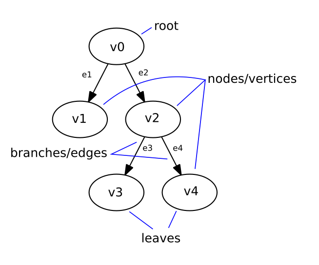
First, a bit of technical background on phylogenetic trees. If a tree starts at a single point of origin, it is said to be ‘rooted’. (Conversely, free floating trees without a single root are ‘unrooted’.) This algorithm will create rooted trees. The fundamental units of these trees are called ‘vertices’ (vertex = singular) or nodes, and the connections between them are called ‘edges’. Nodes can have descendant nodes (or children) and/or ancestral nodes (or parents). The phylogenetic tree example below is rooted at vertex v0 and has edges between the vertices v0 > v1 (e1), v0 > v2 (e2), v2 > v3 (e3) and v2 > v4 (e4).

The nodes at the end of the tree, that do not have children, are the tree’s ‘leaves’ (in the tree below: v1, v3 and v4). They represent the samples, individuals or species that we wish to place on the tree. The internal nodes, sometimes called ‘hidden nodes’ represent the hypothetical ancestral states between two samples or individuals – these are the ‘branching points’ where these two samples diverged (v0 and v2 in the example). In phylogenetics, only these branching points are referred to as nodes, but I will go with the graph theory definition here. Using the example of species evolution, we can think of edges as representing DNA mutations in a species, and the nodes representing either the species themselves, or the hypothetical ancestors between species.

Let’s say we have a matrix *M* with *n* (rows) of samples and *m* (columns) of ‘features’, which denote kind of variation, where 1 can represent the presence of the trait, and 0 the absence. If you’re using genotype data, this might represent whether a locus is homozygous or heterozygous (e.g. 1 = AA or BB, 0 = AB), or this may be a non-sequence based, such as the status of DNA methylation (e.g. 1 = methylated, 0 = unmethylated). The table below shows such a matrix where C1 - C10 are features and S1 - S4 are samples - 1s or 0s representing whether the feature is found in the particular sample.

	C1	C2	C3	C4	C5	C6	C7	C8	C9	C10
S1	1	1	1	1	0	1	1	1	1	1
S2	0	1	1	1	0	0	0	1	0	1
S3	0	1	1	1	0	0	0	0	0	0
S4	0	0	1	0	1	0	0	0	0	0

The Gusfield algorithm implements a test that determines whether a matrix of traits can be represented as a phylogenetic tree, i.e. can we build a tree to explain the evolution of features that are passed down the tree and do not arise spontaneously? This is called the test for a ‘perfect phylogeny’. We define this as a tree T where:

1. each feature corresponds to exactly one edge (and each edge to one feature)
2. each sample has exactly one leaf
3. there is a unique path of edges to any one leaf

The presence of a perfect phylogeny simply denotes that we are able to construct a valid phylogenetic tree where all features evolve down the tree, and ancestral features are not spontaneously re-acquired. To implement the test for perfect phylogeny on a matrix of binary features, we perform the following operations:

1. Discard all duplicate columns in our feature matrix M. Each column is evaluated as its binary number (so for instance, the column C1 with a value 1000 becomes 8; see here for a description of binary numbers). These values are then sorted in decreasing order to determine the column orders. Call this matrix M’ (M prime).
2. Now construct a new matrix k, where each row corresponds to the features present for each sample. Once all the features have been listed, we terminate with a ‘#’ and append 0s for the end of the row.
3. Build the corresponding tree from the matrix and remove the terminating ‘#’ edges
4. Test for the 3 criteria of a perfect phylogeny.

To create our M’ matrix of the feature matrix shown above, we code this up in python like so:

import numpy as np
m = np.array([[1, 1, 0, 1, 0, 1, 1, 1, 1, 1],
              [0, 1, 0, 1, 0, 0, 0, 1, 0, 1],
              [0, 1, 1, 1, 0, 0, 0, 0, 0, 0],
              [0, 0, 0, 0, 1, 0, 0, 0, 0, 0]])

# rotate M for convenient iteration
m_prime = np.rot90(m)

# keep only unique combinations
m_prime = np.unique(map(lambda x: '.'.join(map(str,x)),m_prime))
m_prime = np.array(map(lambda x: map(int,x.split('.')),m_prime))

# count binary score of columns
binary_strings = []
for col in m_prime:
    col_string = '0b'+''.join(map(str,col))
    binary_strings.append(int(col_string,2))

# sort by binary score
order = np.argsort(binary_strings)[::-1]
m_prime = m_prime[order]

m_prime = np.rot90(m_prime[:,:])[::-1] #rotate again
print(m_prime)

Now our M’ matrix looks like:

[[1 1 1 0 0]
 [1 1 0 0 0]
 [1 0 0 1 0]
 [0 0 0 0 1]]

We now have to relabel our features, as duplicate columns have been discarded. The features now become groups representing sets of features that have the same ‘pattern’ of presence and absence between the samples.

	a	b	c	d	e
S1	1	1	1	0	0
S2	1	1	0	0	0
S3	1	0	0	1	0
S4	0	0	0	0	1

To test if a perfect phylogeny exists, we must now construct a matrix k with n rows, where each row lists the features present in each sample, terminated by a ‘#’, followed by ‘0’s (as many as is needed to match the number of columns in M’ ). For example, row S1 [1, 1, 1, 0, 0] has the features a, b, c, so our row becomes [a, b, c, #, 0]. To build the tree, it is convenient to start with the fewest features, hence we can start from the bottom row. We draw edge e, terminate with # and place S4 on the leaf. We start from the root again with S3, draw edge a, d, terminate and mark S3 at the leaf. Now with S2, we follow edge a, then branch out with edge b, terminate, mark S2 and continue this same process for S1.

We can draw the tree in a similar style to the example phylogenetic tree in the earlier part of the post:

This will tell us about how samples S1 – S4 are related. From this result, it appears that S1 only differs from S2 by 1 variant – c, meanwhile it appears that S3 is more related to S2 and S1 than S4.

We can implement the code of constructing matrix k like so:

import string

ncol = len(m_prime[0])
k = np.empty( [0,ncol], dtype='|S15' )
features = np.array(list(string.ascii_lowercase[:ncol]))

for m in m_prime:
    row_feats = features[m!=0] #features in the row
    mrow = np.zeros(ncol,dtype='|S15')
    mrow.fill('0')

    for idx,feature in enumerate(row_feats):
        mrow[idx] = feature

    n_feat = len(row_feats)
    if n_feat < ncol:
        mrow[n_feat]='#'

    k = np.append(k,[mrow],axis=0)

print(k)

a	b	c	#	0
a	b	#	0	0
a	d	#	0	0
e	#	0	0	0

A perfect phylogeny can now be found if each leaf has a unique vector. One way to write this in code, is to determine whether any ‘features’ (a,b,c etc.) are repeated in 1 or more columns of matrix k. Note that the fact that we remove any duplicate columns in an earlier step takes care of the need to test for unique vectors of features leading to each leaf.

locations = []
for feature in features:
    present_at = set([])
    for k_i in k:
        [ present_at.add(loc_list) for loc_list in list(np.where(k_i==feature)[0]) ]
    locations.append(present_at)

loc_test = np.array([len(loc_list)>1 for loc_list in locations])
if np.any(loc_test):
    print 'No phylogeny found!'
else:
    print 'Success! Found phylogeny!'

The matrix above successfully yields a phylogeny:

Success! Found phylogeny!

See my Jupyter notebook for an executable version of this post and the perfect phylogeny repository for a standalone implementation of the algorithm (including an implementation of the imperfect phylogeny algorithm discussed in this post).