The Promethean task of data transfer automation

Long-read sequencing has made signifiant strides in the last several years, with a massive increase in base calling accuracy, bringing it (almost) on par with traditional short-read sequencing. As a perk, it offers methylation calling and cost savings from reusing flow-cells. The unique strengths of the technology also create another side effect—drastically higher data volumes.

Nanopore sequencing allows us to read DNA or RNA from the electrical current fluctuations as the strand passes through a ‘nanopore’—an engineered version of a bacterial protein assembly, embedded in an artificial membrane. The signal is then decoded using deep learning to identify the correct sequence of bases (which also makes it possible to check for methylated base-pairs). This means that the data created via the sequencing machine is in ‘squiggle-space’—containing the raw electrical signal. While Oxford Nanopore Technologies have made strides in reducing the footprint of these data files, they are still typically >1TB per flow cell. Such large data volumes add up—especially in a core facility—and can be tricky to manage.

To add to this ‘feature’, instruments usually have to run as a root user, so IT departments may separate the instrument LAN from the rest of the institute or university’s network. This brings with it extra challenges—how can we get the data from the machine to the researchers most efficiently? We also need to reduce data duplication, have robust error handling, and ensure that the files that were copied from the instrument are the exact files that the researcher receives, and that no files have gone missing in the transfer process. To add to the complexity, once the data has finally made it to the local (non-instrument) network, we then have to make sure that we send the data to the right researcher/lab and their project has enough quota.

When our lab first acquired a PromethION, Nanopore sequencing hadn’t quite reached an inflection point. Handling one or two small runs a month with a few shell commands wasn’t particularly onerous, but as uptake increased, we were quickly seeing several large flow cells being processed every week. Trying to automate the system while it was at this capacity was like rebuilding a car as it is running and gaining speed. The first step was implementing a data transfer form that ensured we had all the information required for a particular transfer. When we were handling requests via email, all the information was dispersed, hard to find, and sometimes hard to untangle from multiple requests. The was a critical step in standardising our process.

Next, we needed a standard for our project folder names. We settled on:

YYYYMMDD_affiliation_labname_projname

This allowed us to sort runs easily by run date on the command line, creating easy separation of external vs. internal runs (by affiliation) and then gave us enough information to send the data to the right lab under the right project name. Including the date was perhaps a bit redundant, as the folder would include run folders generated by the machine with the run date automatically prepended, but it did make it easier to work with projects on the command line. Once this was in place, the first iteration was a simple python script that:

1. Matched project directories via the above pattern—this let us to find the relevant run directories and filter out anything that wasn’t run related.
2. Checked the project directory for completed runs—here we checked for the presence of a sequencing_summary.txt file that was only written to the run directory when the run was complete.
3. Created a tar file of the fastq, fast5 (raw data, later replaced by pod5) and other report/metadata files. Because runs produced many small files, packaging them up aids in the transfer process—as well as being more friendly to the tape system, which is our data’s ultimate destination.

Even this simple script helped tremendously—I could set up a cron job to run every night, and the script would detect runs once they were complete, then tar everything up and package it in a folder, ready to scp to the local network. Half the job was done! Very quickly however, we were running into problems, because the script was tarring everything serially. With the rate of data arriving for transfer, it was just too slow. It was also creating pressure on the available disk space (since we were essentially creating two copies of the data—one version in a tar file and the originals). This data sat there until I could manually transfer it—we needed to transfer it off the machine and delete the tars as soon as possible.

At the time, I had been building pipelines in snakemake, and the parallel-processing nature typical of a standard bioinformatics pipeline ended up being a good fit for the task of processing these data sets. The logic of the archiving process remained similar to the initial python implementation, but now we could process several data sets in parallel. Along with switching to pigz to parallelise the compression/decompression steps, the process was become much more performant! Thankfully the PromethION PC is a beefy machine with a good amount of disk space, so running everything on the machine itself was feasible even with sequencing data being processed concurrently.

Now there was only one bottleneck left to address: transfer from the machine to the local network. One of the biggest issues here was that the machine had to run under a single user with root access (this is often the case with instruments). A ‘service’ user wasn’t an option in this case, so we were stuck for a way to automatically but securely authenticate to the local network using something like scp. This is where Globus came in. Globus is usually used to transfer research data across institutes, but in this case it helped us bridge a significantly smaller gap between the instrument and the local network. As our institute was already set up with a Globus endpoint to our VAST scratch space, it was straight forward to set up an endpoint on our PromethION machine. We could then use globus-automate to move the data to the local network using the copy-and-delete data flow. A bonus of going with this approach is that we could now monitor transfers on the Globus web app. We now had an (almost) automated solution for transferring data from the PromethION to the local network.

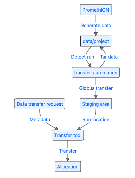
Now that data could be efficiently processed and automatically transferred from the sequencing machine to the local network, there was only one part missing: getting the data to the researcher’s allocation. We were limited to transferring to a scratch staging area. As the final allocation area was not visible to Globus, we had to create another transfer process. In order to make this as easy as possible, we developed a transfer tool using Nextflow that calculated the data volume, checked that the destination existed and had enough quota left, and then performed the transfer using rsync. We also built a validation workflow into this pipeline, so that we could check to make sure that every file that was generated on the PromethION for that particular run made it to the final destination. This tool could be run via Seqera Platform, which we had access to via Australian Biocommons, in order to perform the transfer via GUI. (I also mention this in the talk I gave for Australian Biocommons.) Below is a schematic of the whole process:

PromethION data transfer workflow.

The code for archiving and transferring data from the sequencing machine is available as open source software under nanopore-transfer-automation. While we’re still refining some aspects, all in all, we’ve processed close to 400 runs using this automation approach and it’s saved us lots of time and effort!

Thanks to Rory Bowden for feedback and suggestions for this post.